Data Science using Spreadsheet Software Assignment 3

Printing Workbooks

select the cells you want to print and then set that area as the print area

 

Steps to set a print area:

1. Select the cells: Click and drag to select the range of cells you want to print.
2. Go to Page Layout tab: Click on the "Page Layout" tab in the Excel ribbon.
3. Choose Print Area: In the "Page Setup" group, click on "Print Area".
4. Set Print Area: Select "Set Print Area" from the dropdown menu.
5. Preview and print: Go to "File" > "Print" to preview and then print the selected area. 

Additional Tips:

• Multiple print areas: You can set multiple print areas on a worksheet by holding down the Ctrl key and clicking on the areas you want to print. Each print area will be printed on its own page.
• Clear print area: To remove a print area, go to "Print Area" > "Clear Print Area".
• Print entire worksheet: To print the entire worksheet, ensure no print area is set. 

 

Print Titles –Repeat Rows / Columns

To print column or row headers on every page in Excel, use the "Print Titles" feature. This allows you to repeat specific rows (column headers) or columns (row headers) at the top or left of each printed page, even if your data spans multiple pages. 

Here's how to do it:

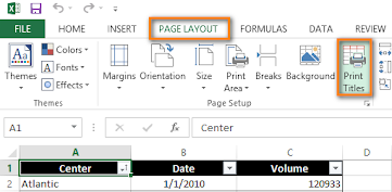
1. Open Page Setup: Go to the "Page Layout" tab on the ribbon, then click "Print Titles" in the "Page Setup" group. 
2. Sheet Tab: In the "Page Setup" dialog box, select the "Sheet" tab. 
3. Rows to Repeat at Top: In the "Print titles" section, enter the reference of the rows containing the column labels. For example, if you want to print the first row on every page, enter "$1:$1". 
4. Columns to Repeat at Left: Similarly, enter the reference of the columns containing the row labels. If you want to print column A on every page, enter "$1:$1". 
5. Confirm and Print: Click "OK" to apply the settings, and then print the worksheet. 

Designing the structure of a template

To design an effective Excel template, start with a clear purpose, organize data logically with descriptive headers, and consider formatting for readability and user-friendliness, saving the file as an Excel template

1. Define the Purpose and Scope:

• What data will the template track?
• Who will use the template?
What are the key insights or actions users need to extract from the data?
Are there any specific formulas or calculations needed? 

2. Structure and Organization:

Organize data into logical sections or tabs.
Use clear and descriptive headers for columns and rows.
Consider using different colors or formatting to highlight important information.
Freeze panes to keep headers visible while scrolling.
Add comments or notes to explain complex formulas or calculations.
Use a consistent style throughout the template. 

3. Formatting for Readability:

Choose a readable font and size.
Use consistent formatting for numbers, dates, and text.
Use borders to separate sections or data ranges.
Consider using conditional formatting to highlight specific data points.







4. Saving as a Template:

Open the workbook.
Click "File" > "Save As".
Choose a location to save the template.
In the "Save as type" dropdown, select "Excel Template (.xltx)".*
Click "Save". 

5. Advanced Features (Optional):

Add VBA code for automation or custom functions.
Insert shapes, images, or charts to enhance the template's visual appeal.
Create dropdown lists or validation rules to ensure data accuracy.
Use Excel's built-in tools for data analysis, such as pivot tables or charts.
Consider using data validation to restrict the type of data that can be entered into a cell.
Use comments to provide instructions or explanations to users. 



Customizing Headers & Footers.

You can add headers or footers at the top or bottom of a printed worksheet in Excel. For example, you might create a footer that has page numbers, the date, and the name of your file. You can create your own, or use many built-in headers and footers.

Headers and footers are displayed only in Page Layout view, Print Preview, and on printed pages. You can also use the Page Setup dialog box if you want to insert headers or footers for more than one worksheet at a time. For other sheet types, such as chart sheets, or charts, you can insert headers and footers only by using the Page Setup dialog box.

Add or change headers or footers in Page Layout view

1. Select the worksheet where you want to add or change headers or footers.

2. Go to Insert > Header & Footer.

   Excel displays the worksheet in Page Layout view.

3. To add or edit a header or footer, select the left, center, or right header or footer text box at the top or the bottom of the worksheet page (under Header, or above Footer).

4. Type the new header or footer text.

Data Science using Spreadsheet Software Assignment 2

 Autocomplete Features

1. Autocomplete: Excel's Autocomplete feature suggests possible completions for a cell value based on the values in the same column.

2. Flash Fill: Flash Fill automatically fills a range of cells with a pattern or formula based on the values in adjacent cells.

3. AutoFill: AutoFill allows you to quickly fill a range of cells with a formula or value.

Using Autocomplete

1. Type the first few characters: Type the first few characters of a value in a cell.

2. Press Enter or Tab: Press Enter or Tab to accept the suggested completion.

3. Use the arrow keys: Use the arrow keys to navigate through the suggested completions.

Formatting Features

1. Number Formatting: Format numbers as currency, dates, times, or percentages.

2. Text Formatting: Format text as bold, italic, or underline.

3. Alignment: Align text to the left, center, or right.

4. Border: Add borders to cells or ranges of cells.

Using Formatting Features

1. Select the cells: Select the cells you want to format.

2. Use the Home tab: Use the Home tab in the ribbon to access formatting options.

3. Use keyboard shortcuts: Use keyboard shortcuts, such as Ctrl+B for bold or Ctrl+I for italic.

Conditional Formatting

1. Highlight Cells: Highlight cells based on specific conditions, such as values or formulas.

2. Data Bars: Display data bars to visualize data.

3. Color Scales: Display color scales to visualize data.

Using Conditional Formatting

1. Select the cells: Select the cells you want to format.

2. Use the Home tab: Use the Home tab in the ribbon to access conditional formatting options.

3. Create a rule: Create a rule to specify the conditions for formatting.

Formatting Tables

1. Create a table: Create a table to organize and format data.

2. Use table styles: Use table styles to quickly format a table.

3. Customize table formatting: Customize table formatting, such as borders and shading.

Using Formatting Tables

1. Select the table: Select the table you want to format.

2. Use the Table Tools tab: Use the Table Tools tab in the ribbon to access table formatting options.

3. Use keyboard shortcuts: Use keyboard shortcuts, such as Ctrl+Shift+F to format a table.

Data Types in Excel

1. Numbers: Whole numbers, decimals, and formulas that calculate numbers.

2. Text: Alphabetic characters, words, and phrases.

3. Dates: Dates and times in various formats.

4. Logical: TRUE or FALSE values.

5. Error: Error messages, such as #N/A or #VALUE!

Data Entry in Excel

1. Typing data: Type data directly into cells.

2. Copying and pasting: Copy data from other sources and paste it into Excel.

3. Importing data: Import data from other files, such as CSV or database files.

Formatting Data in Excel

1. Number formatting: Format numbers as currency, percentages, or dates.

2. Text formatting: Format text as bold, italic, or underline.

3. Date and time formatting: Format dates and times in various formats.

4. Alignment: Align data to the left, center, or right.

5. Border: Add borders to cells or ranges of cells.

Formatting Data Types

1. Formatting numbers: Use the Number tab in the Format Cells dialog box to format numbers.

2. Formatting text: Use the Font tab in the Format Cells dialog box to format text.

3. Formatting dates and times: Use the Number tab in the Format Cells dialog box to format dates and times.

Using Excel's Built-in Formatting Tools

1. AutoFormat: Use AutoFormat to quickly format a range of cells.

2. Format Painter: Use the Format Painter to copy formatting from one cell to another.

3. Conditional Formatting: Use Conditional Formatting to highlight cells based on specific conditions.

Data Validation

1. Restricting data entry: Use data validation to restrict data entry to specific formats or ranges.

2. Creating drop-down lists: Use data validation to create drop-down lists of allowed values.

Data Entry Shortcuts

1. AutoFill: Use AutoFill to quickly fill a range of cells with a formula or value.

2. Flash Fill: Use Flash Fill to automatically fill a range of cells with a pattern or formula.

3. Ctrl+D: Use Ctrl+D to fill down a formula or value.

Number Formats in Excel

1. General: The default format, which displays numbers as they are entered.

2. Number: Displays numbers with a specified number of decimal places.

3. Currency: Displays numbers as currency values, with a currency symbol and two decimal places.

4. Accounting: Displays numbers as accounting values, with a currency symbol and two decimal places.

5. Date: Displays numbers as dates, in a format such as MM/DD/YYYY.

6. Time: Displays numbers as times, in a format such as HH:MM:SS.

7. Percentage: Displays numbers as percentages, with a percentage symbol and two decimal places.

8. Fraction: Displays numbers as fractions, with a specified denominator.

9. Scientific: Displays numbers in scientific notation, with a specified number of decimal places.

10. Text: Displays numbers as text, without any formatting.

Applying Number Formats

1. Select the cells: Select the cells you want to format.

2. Go to the Home tab: Go to the Home tab in the ribbon.

3. Click on the Number group: Click on the Number group.

4. Select the number format: Select the number format you want to apply.

Customizing Number Formats

1. Create a custom format: Create a custom format by selecting "Custom" from the Number group.

2. Use format codes: Use format codes, such as #,##0 for numbers or MM/DD/YYYY for dates.

3. Add formatting options: Add formatting options, such as bold or italic, to the custom format.

Common Number Format Codes

1. #: Digit placeholder.

2. 0: Zero placeholder.

3. .: Decimal point.

4. ,: Thousand separator.

5. %: Percentage symbol.

6. MM: Month placeholder.

7. DD: Day placeholder.

8. YYYY: Year placeholder.

Best Practices for Number Formatting

1. Use consistent formatting: Use consistent formatting throughout your workbook.

2. Use meaningful formatting: Use meaningful formatting, such as currency symbols or percentage signs.

3. Avoid unnecessary formatting: Avoid unnecessary formatting, such as using too many decimal places.

Data Science using Spreadsheet Software Assignment 1

Data Science using Spreadsheet Software Assignment 1 

Excel Interface

1. Ribbon: The ribbon is the topmost part of the Excel interface, providing access to various tools and features.

2. Tabs: The ribbon is divided into tabs, such as Home, Insert, and Formulas.

3. Groups: Each tab is further divided into groups, related to specific tasks.

4. Worksheet: The worksheet is the main area where data is entered and manipulated.

5. Columns and Rows: The worksheet is divided into columns (A, B, C, etc.) and rows (1, 2, 3, etc.).

Basic Features

1. Entering Data: Enter data into cells by typing or pasting.

2. Formatting Cells: Format cells using various options, such as font, alignment, and number formatting.

3. Basic Arithmetic Operations: Perform basic arithmetic operations, such as sum, average, and count.

4. Functions: Use built-in functions, such as SUM, AVERAGE, and COUNTIF.

5. Charts and Graphs: Create charts and graphs to visualize data.

6. Sorting and Filtering: Sort and filter data to organize and analyze it.

7. Copying and Pasting: Copy and paste data within or between worksheets.

Navigation and Selection

1. Cell Selection: Select cells by clicking or using keyboard shortcuts.

2. Range Selection: Select a range of cells by dragging or using keyboard shortcuts.

3. Worksheet Navigation: Navigate between worksheets using tabs or keyboard shortcuts.

4. Zooming: Zoom in or out of the worksheet using the zoom slider or keyboard shortcuts.

Data Management

1. Data Validation: Set data validation rules to restrict input data.

2. Data Formatting: Format data using various options, such as date, time, and currency.

3. Data Analysis: Analyze data using various tools, such as pivot tables and charts.

Simple Spreadsheet

1. Create a new workbook: Open Excel and create a new workbook.

2. Enter data: Enter some simple data, such as a list of names and ages, into the worksheet.

3. Format cells: Format the cells to make the data more readable, such as changing the font and alignment.

4. Basic calculations: Perform some basic calculations, such as summing up the ages.

Basic Spreadsheet

1. Add more data: Add more data to the worksheet, such as addresses and phone numbers.

2. Create a table: Create a table to organize the data and make it easier to analyze.

3. Use formulas: Use formulas to perform calculations, such as calculating the average age.

4. Create a chart: Create a simple chart to visualize the data.

Intermediate Spreadsheet

1. Use functions: Use functions, such as SUMIF and COUNTIF, to perform more complex calculations.

2. Create a pivot table: Create a pivot table to summarize and analyze the data.

3. Use conditional formatting: Use conditional formatting to highlight important data, such as ages above 60.

4. Create a dashboard: Create a simple dashboard to display key metrics and trends.

Complex Spreadsheet

1. Use advanced formulas: Use advanced formulas, such as array formulas and user-defined functions, to perform complex calculations.

2. Create a macro: Create a macro to automate repetitive tasks and workflows.

3. Use data validation: Use data validation to restrict input data and ensure data consistency.

4. Create a dynamic chart: Create a dynamic chart that updates automatically when the data changes.

Advanced Spreadsheet

1. Use Power Query: Use Power Query to import and transform data from external sources.

2. Use Power Pivot: Use Power Pivot to create advanced data models and perform complex data analysis.

3. Use DAX formulas: Use DAX formulas to perform advanced calculations and data analysis.

4. Create a data visualization: Create a data visualization, such as a Power BI report, to display complex data insights.

What is an Excel Template?

An Excel template is a pre-designed spreadsheet that can be used as a starting point for creating new worksheets. Templates can save time and effort by providing a standardized format and layout.

Benefits of Creating Templates in Excel

1. Time-saving: Templates can save time by providing a pre-designed layout and format.

2. Consistency: Templates can ensure consistency in formatting and layout across multiple worksheets.

3. Easy to use: Templates can be easily shared and used by others, even those with limited Excel experience.

Steps to Create a Template in Excel

1. Create a new workbook: Open Excel and create a new workbook.

2. Design the template: Design the template by adding the necessary columns, rows, and formatting.

3. Add formulas and functions: Add formulas and functions as needed to make the template more dynamic.

4. Format the template: Format the template to make it visually appealing and easy to use.

5. Save the template: Save the template as an Excel Template (.xltx) file.

Tips for Creating Effective Templates

1. Keep it simple: Keep the template simple and easy to use.

2. Use clear headings: Use clear headings and labels to make the template easy to understand.

3. Use consistent formatting: Use consistent formatting throughout the template.

4. Test the template: Test the template to ensure it works as expected.

Using Excel Templates

1. Open the template: Open the template file (.xltx) in Excel.

2. Save as a new file: Save the template as a new file (.xlsx) to create a new worksheet.

3. Enter data: Enter data into the worksheet, using the pre-designed layout and format.

Sharing Excel Templates

1. Share via email: Share the template via email by attaching the template file (.xltx).

2. Share via cloud storage: Share the template via cloud storage services, such as OneDrive or Google Drive.

3. Share via network: Share the template via a network, by saving it to a shared drive or folder.